Newton's Mechanics
The K vector shows the direction of the movement of the pendulum. It can be defined as |K| = mgsinα. Consider the displacement of the mass at the end of the pendulum as x. So the vector K remains as:

We know the value of the displacement x and its second derivative as:


If we substitute those values in the precedent equation, and making the approximation of the sinus for small displacements of we get:

Solving this differential equation of order 2, we get:

Lagrange's Mechanics
Here, we must first find the kinetic and potential energies:


With those energies, we can obtain the Lagrangian:

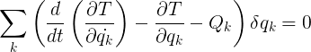
Now we can apply the Lagrange's equation to obtain the motion of the pendulum:


This is the same differential equation as the one get with the Newtonian mechanics.
Hamilton's Mechanics
We start from the Lagrangian, and the generalized momentum:
Now, with the value of the generalized momentum, we can substitute the derivative of α from the Lagrangian and get the Hamiltonian:


If, now, we apply the Hamilton's equations:

Substituting the values of the generalized momentum, we reach to the same differential equation as in the two other cases; with the same final result.
Conclusion
As you've see, the three methods hopefully gave the same result, which confirm that they are a reformulation of the same mechanics. The Newton's mechanics is more simplistic, and for problems with more constraints, you must deal with a system of several equations.
The Lagrangian's mechanics reduce the number of equations to the number of constraints. This is the method with less equations to solve, but you must deal with almost a differential equation of order two.
And the Hamiltonian's mechanics have twice the number of equations than the Lagrangian, but you with easier calculus, as the Hamilton equations does have second degree derivatives.