C - Introduction

C is a programming language used in many fields. It's a low-level language, which means that you will handle some low-level computer features as the memory usage. It's used in many microcontrollers as it requires a minimal installation and runtime support. Other programming languages (as Java) will need a virtual machine which will run the application, with C, at compile time, the runnable application will be build in a machine language yet, so less memory consumption will be needed by the machine (as it don't need a sideway application as the virtual machine), and less stockage too (as no virtual machine must be installed).

How to build an application with C? When you write the commands you want to run in your application, you will do it in a text plain format file (ASCII encoding), with this file (or a set of files), you will call the compilation program which will build your application (gcc, https://gcc.gnu.org/). This will build your application in four steps:

1. Preprocessing. Basically, it will put all your written program in a single file; this is, every time you wrote #include it will include the given file. It will also concatenate all the single lines you broke for readability.
2. Compilation & Assembly. It will traduce your text plain format file into a machine language format. This is one of the most important steps, where you will know if you made some syntax errors the machine don't understand. Also, the result of these step will be machine specific; you can't build your application in a Linux platform and try to run it on a Windows. The compilation step will build an intermediate human readable result, and the assembly will build a machine code.
3. Linking. This is the last step. It will include all the generated code into a single runnable file. It will include all your psot-compiled files, and additional required libraries. This will result in a single runnable file.

Let's see a simple example: a "Hello World".

For the current simple example, I've used no IDE, only a simple text editor (vim) and the compilation was made in a terminal with gcc in a Linux platform. The example shown, is composed by a standard library import at the first line (this import some basics commands as the printf). In the line 3 we declare the main entry point of the application. This is needed in all the application by the compiler a to know where the application must start. Without this declaration, your machine will not know at which instruction start. The main method declaration can be more configurable (with inputs) but for the current example, it's enough. At line 4, we use the instruction printf which will print in the output console the message given as the argument (in this case "hello world"). The final character \n means that a new line will be printed at the end of the text, otherwise, you will continue with the cursor at the end of the current line. And finally, the return 0; at line 5 indicates the return code of our application. The value of 0 is mainly used to indicate that all went good (it's only a convention, not a rule); and negative values indicate different kind of errors (each one will be defined by the user as it needs them).

After writing this application in a file named helloworld.c you can compile it with a terminal:

We can see that we start with our single file helloworld.c. Then we use gcc to compile and generate our runnable application. gcc accepts as first argument a list of file which you want to compile, and with the -o parameter, we specify the file of the output we want. The output will be the generated runnable application, which can be run as shown in the figure.

Compile your application with a terminal can be a big headache, as your application grown you will have more and more files. The best option (also for edition) is to use an IDE, in the next articles I'll use Geany (https://www.geany.org/) which is a lightweight IDE. The IDE use to help you for both compilation and edition of your applications, as the compilation will be automatic (it will detect the files you included in your project to add them at the compilation time) and you can have some useful autocomplete when editing.

Maxima - Interpolation

In science, you often have to made analysis of a set of data, a huge set of data. There are many analysis you can do with them, but an interesting thing you can do with an application like Maxima, is the interpolation to know the value of intermediary or external values of the given set. In this article, we'll see four methods: the lineal interpolation (with the command linearinterpol()); the spline interpolation (with the command cspline()); the Lagrange interpolation (with the command lagrange()); and the least squares (with the command lsquares_estimates()). As said before, I'm not going to explain the mathematical methods, but only how to use them in an application like Maxima.

The three interpolation methods (the lineal, spline and Lagrange), can help you a lot when you desire is getting a value in the middle of the set of data. But when you're trying to find a value outside the limits of your set, you'll have a more accurate result with the lest square method (depending on the variation of the function near the limits of our set). The interpolation methods need a specific package to be imported before use them:

After that, the three functions are available for use. Both three methods, only have a single input argument, the set of data, and as an output, you will have a function which defines the interpolation. Let's see an example with the three usages:

As you see the usage is quite simple. Let's see the result:

For this particular example (with so few points), we see that both the three methods converge quite well to the function (which was similar to 2*sin(x)).

Let's now see the fourth method, the least squares method. This function also requires a particular package to be imported (load(lsquares)$). The usage of the least squares method is different from the others. You must have an idea of the curve your set represents, with some unknown values. The inputs for this functions are different from the others. First, it needs a matrix, not a list of value. The matrix will have the values for each variable per row. Second, we specify which variable corresponds to each row of the matrix. Third, the model which represents (approximately) our function with the unknown values. And fourth, the list of the unknown values. Let's see the previous example with this method:

In the first line, we load the required package to use the function lsquares_estimates(). The second line, show our data, and the next how we insert it in a matrix with another row with only indexes starting at 0. Then we transpose the matrix to have the values per row as a set of key-value. We then use the lsquares_estimates() and stores its output. The output are the values of the given unknown constants A, B and C, which we make the substitution on our approximate model, and finally plot the result.

Maxima - Differential Equation

Solving differential equations can be very tricky when doing it analytically, it's the same for a mathematical application as Maxima, which can't solve differential equations which have an order higher than 2. There is also a big complexity to solve partial differential equations. But when you lead to a differential equation which can't be solved analytically, you always have the numerical methods as Runge-Kutta. You must take into account that the mathematical applications will mainly be used to obtain numerical as it's easiest to compute, and at the end you're more often looking for a numerical value.

Let's take a look over the differential equations functions: ode2() to solve differential equations of order 1 or 2; ic1() to solve differential equations of order 1 with initial values; ic2() to solve differential equations of order 2 with initial values; and bc2() to solve differential equations of order 2 with boundary values. Well, the functions exists, but how to use them? ic1(), ic2() and bc2() have as inputs a general solution given by ode2(). This means that the amount of equations which can be solved is reduced. But we always can use some analytics way to transform a higher order differential equation into a differential equation of order 2 with a separation of variables. But this leads that the differential equations which can be solved are only the one which have initial values (not the boundaries values).

Let's try to see all the resume into a single exercise:

Solve numerically for 0 < t < 50 this system of differential equations:

 

Here are the initial values:

 

For the Runge-Kutta method, take steps as 0.1.

As we want to use the Runge-Kutta method as the numerical method to obtain all the data of the given equations, we need to have a system of differential equation of order 1. To do so, we will do a change of variables introducing u(t) and v(t) as follows:

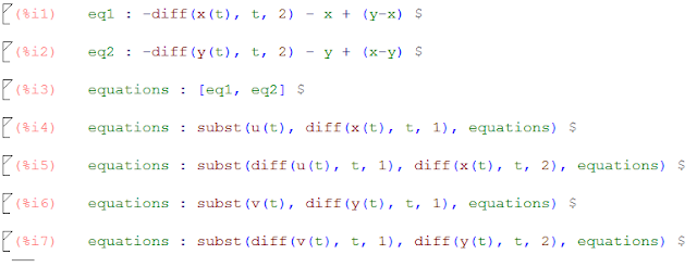
Let's see each lines in details. The first two inputs are the given differential equations written as f(x, y) = 0. In the third input, we create a list with all the equations, where we will add the two new definitions of u(t) and v(t) later. In the forth and sixth, we define the u(t) and v(t) as the derivatives of the functions x(t) and y(t) respectively. And in the fifth and seventh inputs, we make the substitution of the new functions in our differential equations. Now we're with system of differential equations of order 1.
Then we prepare the inputs for the rk() function.

In the input 8, we add the definition of u(t) and v(t) to our list of differential equations. We add them as the previous, as f(x, y) = 0. In the input 9, we sum our list of differential equations with derivatives of each dependent variable, having this way the prepared input for the Runge-Kutta function. And in the input 10, we substitute the variables without the term t (the (t) was necessary for the derivatives functions, as it needs to know who depends on who). We build the missing inputs for the Runge-Kutta function in the inputs 11, 12 and 13 as the list of the dependent values, the list of the initial conditions, and a list with the independent variable and its range. Then we call the function rk() and store its output.

Now we can get the results to plot them:

First we apply the matrix function to the rk() output, then, transposing the matrix, we can get the independent values for each variable, t, x, y, u or v. 

Let's see now some graphs. First at all, the two initial differential equations are from a system of 2 coupled harmonic oscillators. So, if we plot x vs t and y vs t we can see the position of the 2 harmonic oscillators:

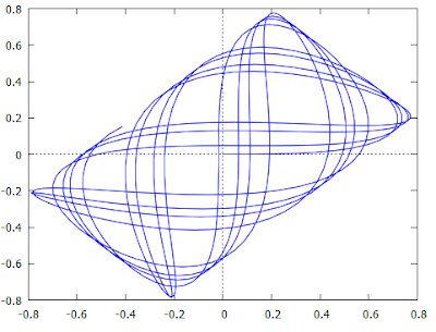
Another interesting graph, is if we plot y vs x, which is known as the Lissajous figure:

And finally, we can plot the speeds vs the positions (u vs x and v vs y):

This is also known as the phase diagram of the system.

Maxima - Analytics solution

When you have an equation as F(x, y) = 0, this is an implicit solution of the equation. Sometimes you can solve this equation for y, but only if the function satisfy the implicit theorem (https://en.wikipedia.org/wiki/Implicit_function_theorem). If the equation does satisfy the conditions of the theorem, you can solve it as y = f(x). 

How to do that with Maxima? First, we will use the function solve() to obtain all the solutions of the given equation. The solve() function will give you all the available solutions if there are, or none if it can't. Then we use the output of solve() as input for sublis(). 

What does sublis()? It substitute a list of given values into a given equation. When we get the solutions with solve() we do the substitutions of the solutions by y.

Let's see an example:

 

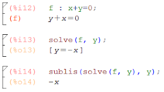
 Here we defined f as an equation. With solve() we solve the equation f for y. In this example we only have a single solution, but solve() will give us all the existing solutions in a list. And finally, we give the output of solve() to sublis() to get y solved.

The previous example is too easy. Let's make a generic function which leads with multiple solutions given by solve().

 

 Here we iterate with a for loop over all the solutions given by solve(), and at each step, we append a new y solution to our list which will be returned as our output.

 This procedure can only be used if the function f satisfies the implicit theorem. Otherwise, we must solve the equation with numerical procedures.

Maxima - Plotting

Maxima is also a powerful plotting application (for both 2D and 3D). In this article, I going to introduce you to commands plot2d and plot3d. Both functions are very similar concerning the needed inputs, consequently, all the example I'm going to show are about plot2d but can also be applied to plot3d. As input, it needs: the function you want to plot; the limits of the plot (for 2D, the x limit is mandatory, but not the y limit, but you can also specify it (it's interesting if you got infinite values at y)); and some options (color, logarithmic scale, line style, labels...). Let's see some examples.

We start by plotting the sinus functions:

There isn't complicated. There is the sin(x) argument as the function input (we could use another variable as phi or alpha, but you'll need to add it in the second input); and then the x range (minimum and maximum). Pi is a Maxima constant, that's why I used the "%" symbol just before, otherwise Maxima will interpret it as a new variable named pi. There are a lot of constants in Maxima, and when you want to refer to one of them, just add "%" before (and check in the online manual the constant actually exists). 

Let's continue with the same example:

 

 Here I've added some useful options: first, I've increased the x range by multiplying by 2 the inferior limit; I've also added the y range; I've added the color of the line; and the labels for both the X and Y axis.

 And for plotting multiples functions in the same image?

 The function plot2d also accepts a list of functions as first input. But you will need to adapt all your options: you will need two colors as there are two lines; and two legends, if I haven't added the legend option, the legend will be the function itself (it's very useful for large functions to avoid having the entire function as the legend).

 And for plot3d?

Same as plot3d, I'm not going to explain again the inputs.

And now a practical exercise:

 Plot a function and its corresponding Taylor series near to a given point and for a given grade.

This is a very interesting exercise, as now you will see how the Taylor series is more accurate as you increase the grade. The function to obtain the consecutive Taylor series, was yet done in a previous article (https://physicsisbeautiful.blogspot.fr/2016/06/loops-conditions.html), so let's do the plotting part. We will use the previously said function inside our plotting function.

And here the plotting function:

First, we stock the results of the taylor_grade_n() function into a list. Then we use the plot2d() function to plot the results, but in the functions input of plot2d we must also add the original function, this way we can see the difference between the original and the Taylor series. And the last argument is that we disable the legend, as the higher grade of the Taylor series will be a large function. We could have done a legend with the grade of each function, but I let you doing this.

Maxima - Loops & Conditions

Here, I'll explain two very important tools used in every programming language. The loops and conditions. When you're creating an application, the way you want the application to be executed is not always linear, but you'll want your application to go one way if... or another way if... You also could want to perform a single manipulation a repeated amount of times. Let's see some examples:

I think the code is easy to understand. The main statements here, are if, then and else. With if you specify the condition, you can specify an equality (=), a comparison (>=, >, <, <=) or an inequality (!=). With then you start the statements you want to execute if the if-condition is satisfied, you can add as many as you want. And finally, the else statement define the code which will be executed if the if-condition is not satisfied. Let's continue with a more complicated example:

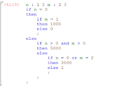
As you can see, the if-condition can have multiple conditions, separated with and or or as logical operators.

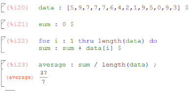
The for loops. When you want to run a task a determined amount of times, you can use the for loops. Those loops are build with three parts: an initial part where you specify the variable which will behave as the index, and its initial value; the final condition until when the loop must be executed; and the steps the index must be incremented at each loop. Let's do an example: give the average of the elements in a list (this can be done directly with another instruction, but that's not what we want to test today):

In some cases, you could want to have another for loop inside the first for loop, but this must done with caution, as the execution time increase exponentially. If you have three for loops, and the elements to handle are 10 or 12, your code will be executed 1000 or 1728 times (a difference of 728 just adding two elements to the original list).
There are some variants of the for loop, you can specify an iteration from an initial value to a final value (with thru); a condition which must be satisfied to iterate the loop (with while); or a condition which must not be satisfied to iterate the loop (with unless).

Let's continue with a simple exercise:

Write an application which gives the Taylor series of a function for a grade from 1 to n.

To solve this problem, we can just do a for loop, and make the Taylor series of the function from 1 to n, but if n is high, this could cost a lot of execution time. Let's examine the Taylor series: it's the consecutive derived of a function. So if we do manually the derived from 1 to n, we have at each loop step a new solution. Let's see the code:

Our function is called taylor_grade_n with the inputs: the function, the points where to get the Taylor series, and the grade. We start by saving the function in an temporal variable to avoid modify the input value. Then we stock the first value (the function without any derived) in a list, which we will append the rest of the values in the for loop. At each step of the for loop, we append the previous value of the result list with the new derived multiplied by (1/index!)*(x - x0).

Maxima - Linear Algebra

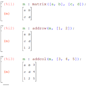
Let's see more in details the matrices and operations with matrices. As we saw previously, the matrices are in fact a list of lists of values, each list is a row. The amount of list is the amount of rows, and the amount of elements in a list is the amount of columns (each list must have the same amount of elements, otherwise you will get an error). Let's try to change the size of a matrix:

First, each statement describe quite well the action he do, so try, when we create our own functions, to describe the best as possible the function by the name. If there is a Maxima command which we don't know what it does, or what it expects as input, just write describe(xxx); and Maxima will show you the documentation of the desired function.

Second, when adding rows or columns, be aware to adding the same amount of elements as the matrix accepts. We can see that when adding the row, it has 2 elements, but when adding the column it has 3 elements.

Third, the functions addrow() and addcol() don't modify the original matrix, that's why we need to save the output of those function to m. There are some function which modify the input but isn't a good practice, as you could need to save the result to another variable, maintaining the first matrix unchanged.

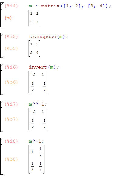
Let's continue with some other matrix operations.

 

 The transpose and invert operation of a matrix can be very tedious, but as we can see, with Maxima is easy. There is two ways to obtain the inverted matrix: using the command invert() or elevating the matrix to -1. Be aware with the second method, because if  want to obtain the inverse of the matrix, you must write it as m^^-1, but if you want to obtain the inverse of each element of the matrix, you must write it as m^-1.

We can continue with some other basics operations.

 

 First, we've created another matrix to play with. In the first operation (input 10), we've added the value 1 to each element of the matrix. At the input 11, we've made the sum of two matrices, having the result as the sum of each elements of each matrices. At the input 12, we've multiplied two matrices, having the result at the first row/first column as m1[1][1] * m2[1][1] + m1[1][2] * m[2][1] (the classic matrix multiplication). And at 13, we've the multiplication of each element of both matrices placed at the same position. You remember the difference between those two multiplication signs.

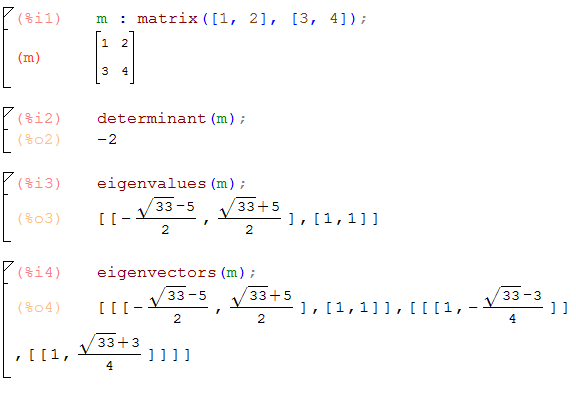
And now the eigenvalues and eigenvectors.

As we saw before, the functions determinant(), eigenvalues() and eigenvectors() accept a single input and return an output without modifying our input. For the eigenvalues and eigenvectors we have a list as a result (a list of vectors for the eigenvectors).

Let's solve a simple problem:

Write a function which rotate tridimensional objects. 

inputs:

• A list of points which define the object to rotate
• The three Euler angles
• The center position from where the rotation must be made

output:

• A list of points which define the rotated object.

 As this article is mainly based on the Maxima application, I will not explain in details the mathematical part of this problem. To obtain the result, we must first create the Euler matrix with the given angles. Then apply the rotation matrix to the given points. We also must take into account the center of rotation. So the main equation remains as center + rotation . (points - center). I've used the "." multiplication sign as it is the one used by Maxima for the matrices multiplication. Let's do this in a block, this way we can use it later easly.

Let's analyze this piece of code. At the first line, I've declared the function with all the inputs and the inner variables we will use inside the block. When you're developing an application like this, it's hard to know at first time the inner variables you will need. Those are added as you're writing the code inside the block (with some practice, you will understand). In the third and fifth lines, I've created two temporary matrices to build later the Euler rotation matrix. At seventh line is the Euler rotation matrix. At ninth, I've created an intermediary matrix to avoid using parenthesis in the last line (to maintain the code more readable). And finally, at the last line, the equation we wanted.

Maxima - Introduction

Maxima (http://maxima.sourceforge.net/) is a mathematical program to allow you to solve multiple type of equations. It has a syntax very similar to many programming languages (Java, C++, Python..). In this article, I will introduce the basic usage to allow later solving more complicated equations. I will not explain in details the mathematical concepts, I will mainly base this article on the programming language. The program I use is WxMaxima (http://andrejv.github.io/wxmaxima/), but I've used it without any help purposed by the program, I could have done the same with the command console of Maxima.

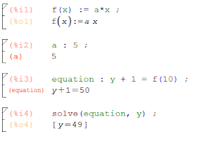
When starting the WxMaxima application, we see an empty command console. What's a command console? It's a non graphical interface where the user can introduce instructions to an application which will be executed when we introduce the final character of our instruction. What's an instruction? It could be a sum, subtraction, variables assignation, functions creation, equation solving... Normally, it's what we introduce in a single line (but you also can introduce multiple instructions per line). The instructions can have one input parameter (the variables we pass between parenthesis), multiples inputs or none. And each instruction we return some output data. Some will return nothing (as the assignation of a value to a variable), and some will return a simple or complex structure of data (the sum will only return the result of the sum, but when transposing a matrix we will get the transposed matrix as the result). How to tell the program the end of our instruction? With WxMaxima, you can do it with Ctrl+Enter. This will add the character ";" at the end of the line and print the output. If you don't want (don't need) the output, use the "$" character instead (the instruction will be executed too). When will I don't need the output? When you set the value 5 to the variable x, you don't need the program to tell you that you assigned the value 5 to x. When you want to save the definition of equation into a variable, it could be interesting to see the result, to confirm you didn't made a typo. What can I save into a variable? Whatever you want. Numerical values, text (a single word or a complete sentence), equations or functions (I will explain later the difference between both), list of data, list of lists (a matrix)... How do I do the assignation? There is 3 ways to do an assignation depending on what you want to assign: ":", "=" or ":=". To assign a value to a variable, use ":". After this assignation, the variable will have the behavior of the numerical assigned value. This is useful when you need to create/introduce an equation which needs constants (as the permittivity of vacuum, the mass of the electron...). For equation, use "=". When you write an equation where you want to take off the value of a variable, use the "=" in the equation. And finally, ":=" is used for the function assignation. When you want to create a equation where you must specify the input and then you get the output, this is a function. Here is an example of the 3 cases:

Each line starts with a (%iN), this means the N input we've made. And the output will be (%oN). In the first input, we've created the function f(x) as a*x (the multiplication sign is mandatory, otherwise it will consider a variable named ax). From now we can use f(x) instead of a*x. In the second input, we've assigned the value 5 to the variable a. This way f(x) will remains as 5*x. In the third input, we've created an equation where we want to know the value of y. And in the last input, we've used the Maxima instruction solve to solve our equation. The solve instruction has two inputs, the first is the equation you want to solve, and the second, is the variable you want to know the value (you can have more information at http://maxima.sourceforge.net/docs/manual/maxima_20.html or writing describe(solve); in the application). If we've used the final character ";" instead of "$", the final result wouldn't change:

 

Lets continue with some useful commands:

Comments: when you're writing complicated and long formulas, sometimes (or always) you need to explain some steps of your formulas. Here you can do it so. The comments start with /* and end with */. They can be at the beginning of the instruction, at the end, or in the middle.

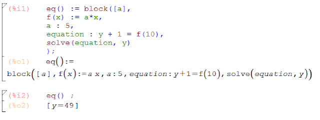
 Blocks: if you have to build a complex and long equation, you can use variables to stock some constant values, or divide your equation in some little steps. When using constants, imagine you use the names a, b and c for the first equation, lets continue with the second equation with d, e and f. If you continue that way, you will mix some constants with the equations. Using blocks, you can have your own a, b and c variables for each equation independently (the naming strategy should be better and more descriptive). Lets see an example.

First, we see that all the information in the block is stocked into a variable eq() (having parenthesis it's now a function). In this case, we've made a function without inputs, if we need some inputs, they will be declared into those parenthesis.

 

After the block command, we define a list of variables used inside our block, which won't have any meaning outside the block. Then all the instructions which must be used inside the block coma separated (this time we only use the final character when closing the block statement). When editing, we can push Enter to have a new line an have a better readability of our block, Maxima won't compute anything, as it's still missing the final character. And to execute our function, we only have to write eq() and Maxima will execute all the instructions inside our block. When you're asked to write a block with a specific behavior, is quite hard to write is as you see in the picture (from up to down) in one shot. You must first try to decompose the behavior is small parts that you better understand. Dividing a huge function in small parts is always better, as you read it better (for you and for other people), it's better to understand its behavior and repair it if necessary, and more suitable to write and comment.

List and matrices. And finally, I will introduce the data structure used in Maxima. The list and matrices are the most used for inputs and outputs. You can create a list only by typing the symbols "[" and "]" separating each element by ",".

 As you can see, the list can have multiple type of data (this isn't a good practice). And if you want to access to a single element inside the list, you just have to put the index of your element between "[]". For matrices, it's very similar. As it's considered as a list of lists, but you've a specific command to create them.

 The matrix command is used to create a matrix directly, you just have to specify as input the list of values present at each line.