Maxima - Differential Equation

Solving differential equations can be very tricky when doing it analytically, it's the same for a mathematical application as Maxima, which can't solve differential equations which have an order higher than 2. There is also a big complexity to solve partial differential equations. But when you lead to a differential equation which can't be solved analytically, you always have the numerical methods as Runge-Kutta. You must take into account that the mathematical applications will mainly be used to obtain numerical as it's easiest to compute, and at the end you're more often looking for a numerical value.

Let's take a look over the differential equations functions: ode2() to solve differential equations of order 1 or 2; ic1() to solve differential equations of order 1 with initial values; ic2() to solve differential equations of order 2 with initial values; and bc2() to solve differential equations of order 2 with boundary values. Well, the functions exists, but how to use them? ic1(), ic2() and bc2() have as inputs a general solution given by ode2(). This means that the amount of equations which can be solved is reduced. But we always can use some analytics way to transform a higher order differential equation into a differential equation of order 2 with a separation of variables. But this leads that the differential equations which can be solved are only the one which have initial values (not the boundaries values).

Let's try to see all the resume into a single exercise:

Solve numerically for 0 < t < 50 this system of differential equations:

 

Here are the initial values:

 

For the Runge-Kutta method, take steps as 0.1.

As we want to use the Runge-Kutta method as the numerical method to obtain all the data of the given equations, we need to have a system of differential equation of order 1. To do so, we will do a change of variables introducing u(t) and v(t) as follows:

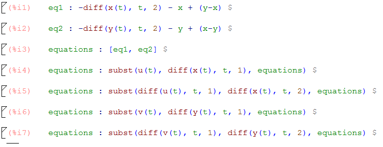
Let's see each lines in details. The first two inputs are the given differential equations written as f(x, y) = 0. In the third input, we create a list with all the equations, where we will add the two new definitions of u(t) and v(t) later. In the forth and sixth, we define the u(t) and v(t) as the derivatives of the functions x(t) and y(t) respectively. And in the fifth and seventh inputs, we make the substitution of the new functions in our differential equations. Now we're with system of differential equations of order 1.
Then we prepare the inputs for the rk() function.

In the input 8, we add the definition of u(t) and v(t) to our list of differential equations. We add them as the previous, as f(x, y) = 0. In the input 9, we sum our list of differential equations with derivatives of each dependent variable, having this way the prepared input for the Runge-Kutta function. And in the input 10, we substitute the variables without the term t (the (t) was necessary for the derivatives functions, as it needs to know who depends on who). We build the missing inputs for the Runge-Kutta function in the inputs 11, 12 and 13 as the list of the dependent values, the list of the initial conditions, and a list with the independent variable and its range. Then we call the function rk() and store its output.

Now we can get the results to plot them:

First we apply the matrix function to the rk() output, then, transposing the matrix, we can get the independent values for each variable, t, x, y, u or v. 

Let's see now some graphs. First at all, the two initial differential equations are from a system of 2 coupled harmonic oscillators. So, if we plot x vs t and y vs t we can see the position of the 2 harmonic oscillators:

Another interesting graph, is if we plot y vs x, which is known as the Lissajous figure:

And finally, we can plot the speeds vs the positions (u vs x and v vs y):

This is also known as the phase diagram of the system.